Example 3
Modification of building model
The example carries on with the building description and data model described in the examples EX1 and EX2. It is assumed that data of these models have been saved as a basis for this continuation. The building model is complemented with data for the following conditions:
shadows from the surroundings
replacing the glazing type with a low energy glazing
solar shading for the windows
ventilation systems
On the basis of the completed building model, a one year's simulation is carried out, and the energy and indoor climatic conditions are compared with the results from example 2.
Read existing model and copy to a new name
Fetch the building model EX2 into BSim and save under the name "EX3" as described in example 2. The new model (the file EX3.DIS) is then used for further extension of the building model.
Description of shadows and typing in the data
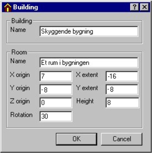
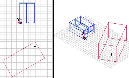
The windows in the actual building lie partly in the shadow of another building, which is situated to the south, at a distance of 8 meters, is 8 meters high, and stretches 16 meters and have a rotation of 30 ° compared to the East-West axis (the X-axis), as shown in the figure below.
Typing in data for shadows
The external shadow is described by inserting a new building in the model. This can happen either as an existing project or by creation of a new building - which is done in this example. Double-click in the plan drawing (marked as a cross) to select a reference point where the new building is to be drawn from. Select Add Building from the SimView menu. If the reference point is not located 100 % correct, the correct co-ordinates can be input in the building dialog:
This creates a new building in the model. The new building will cast shadows on the existing building when simulated in tsbi5.
Selection of another type of glazing
In order to examine the significance of the thermal resistance of the glazing on the overall heat requirement, the type of pane used is to be replaced by a super low energy pane. The database is opened (click the database-button in the job list or click the SimDB icon in the toolbar) and the entry External is selected in the BuildingElement part of the database. The entry "SuperLavE-Kr i træramme" is selected. The SfB-number is selected and drawn to those windows that should have the new type, and the SfB-number is released here. It is also possible to use the Defaults entry of the SimView menu, as described in example 2.
Solar shading for the windows
In order to reduce the solar radiation through the windows and to limit overheating of the building during the summer, solar shading devices are fitted to both windows. Right clicking a window in the tree structure shows the WinDoor property dialog:
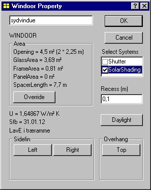
Placing a tick-mark next to SolarShading adds the system solar shading to the window. In the tree structure one can now right-click SolarShading to open the solar shading dialog for the actual window:
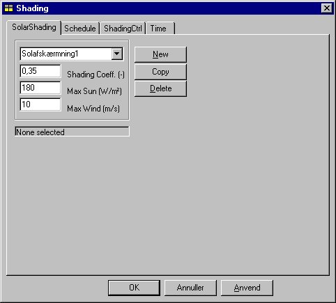
For the shading coefficient - Shading coeff. - the value 0.35 is entered, corresponding to an internal, white curtain. Note that "shading coefficient" is a popularly accepted designation, which is defined as the relationship between the solar radiation through the pane with solar shading and the solar radiation through the pane without solar shading (between 0 and 1). The name is thus somewhat misleading, since it expresses how much radiation passes through the solar shading (and not how much is shaded) so that a low figure is an expression of effective shading.
The second parameter which must be entered for the shading is Max Sun, which indicates a limit for the solar radiation through 1 m² of the current window, above which the solar shading is activated. The value of this parameter must be selected with regard to the total window area, the solar shading for the remaining windows in the zone as well as the shape of the zone and the placing of work places in relation to the windows.
Direct solar radiation, which strikes persons in the room, is normally considered to be uncomfortable. Transmitted diffuse solar radiation from the sky and reflected radiation from surroundings will seldom exceed 150 W/m², and it can often be assumed that the limit will lie between 100 and 200 W/m². In this case, the value is entered as 180.
The field Max Wind indicates the maximum wind speed at which the solar shading can be in action. For instance it can be awnings, which can not stand wind speeds above 10 m/s.
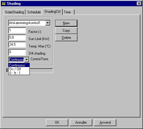
On the tab ShadingCtrl the control of the solar shading is defined:
Direct solar radiation, which strikes people in the room, is normally considered to be uncomfortable. Transmitted diffuse solar radiation from the sky and reflected radiation from the surroundings will seldom exceed 150 W/m², and it can often be assumed that the limit will lie between 100 and 200 W/m². In this case, the value is entered as 180.
Solar shading control
The schedule for solar shading makes it possible to define several different forms of control. The shading factor defined in the shading dialog will normally express how effective the solar shading is, when drawn fully across the window. In the Shading control tab, the first field Factor makes it possible to indicate that the solar shading, within the connected time definition, is not drawn completely.
The values of the next two parameters in the dialog Sun Limit and Temp. Max together define a strategy for activation of the solar shading, when it is too hot in the thermal zone. Temp. Max indicates an upper limit for how high a temperature can be accepted, before the solar shading is drawn. Sun Limit indicates a minimum total solar radiation through all windows, which is admitted to the thermal zone, before the solar shading will be used to reduce the temperature at all. This limit is set to avoid unnecessary (or absurd) control of the solar shading at times (e.g. at night) where the solar incidence is very small, and where solar shading control therefore cannot reduce the indoor temperature.
In this case the value 0.8 (kW) is entered. The total window pane area for the two windows is approx. 7.4 m² (2 x 1.8 x 2.05) and the sun limit therefore corresponds to approx. 108 W/m². For the temperature limit, Temp. Max the value 24.5 (°C) is entered.
This means: First the program checks if the solar radiation at the internal face of the WinDoor exceeds the limit of 180 W/m². If this is the case, the solar shading comes into use, depending on the Control Form given at the ShadingCtrl tab. Then the program checks if the operative temperature in the thermal zone is above 24,5 °C and if the total solar incidence through all WinDoors in the thermal zone exceeds 800 W. If this is the case the solar shading comes into use, depending on the Control Form, in this case just so much (as Continuous control is selected) that the limit - if possible - for the operative temperature is maintained.
The last input field, SF4 shading, defines the "solar light factor" for the window, when the solar shading is completely drawn. The solar light factor is defined for a given reference point in the room, and expresses the ratio between the daylight illuminance level at the reference point and the simultaneous illuminance outdoors on the surface of the facade, cf Algorithms for calculation of solar radiation and daylight.
For unshaded windows, the solar light factor will normally vary considerably through the room, from a magnitude of 0.20 - 0.15 close to the window to a magnitude of 0.02 - 0.005 at the back of the room. The factor SF4 for a shaded window is defined for a "window" with transmittance 1, as the reduction of the transmittance for window pane and solar shading is accounted for in the data for window pane and shading, respectively.
Note that whilst the illuminance at any point in the room is reduced proportionally with the light transmittance figure for the window and with (1 - the solar shading factor) for the shading, the solar light factor expresses at a given point in the room, how much the illuminance at precisely this point is changed by using the solar shading. The average illuminance in the room will always drop when the solar shading is drawn, but some types of shading (e.g. reflective Venetian blinds), which even out the light variation throughout the room, so that the illuminance is increased at the back of the room, when the solar shading is used. The purpose with such shading is to reduce the illuminance difference (which can cause uncomfortable glare) by the window and at the same time to improve the daylight utilization at the back of the room, so that the need for artificial lighting is reduced.
When the solar shading is partly drawn for the window, the daylight illuminance at a given point is calculated as a weighted value of the illuminance for portion of the window which is shaded and the illuminance of the other, unshaded part of the window.
In the present example, it has been decided to let the artificial lighting be controlled simply according to the solar radiation through the windows (cf. example 2) and the value of the solar light factor SF4 will therefore not be used. The general principle is, however, that all parameters for components and systems used must be assigned a value, so here the value 0 is entered.
Control strategy
The last field in the dialog for shading control is the access to a selection menu in which it must be defined how the shading is used. For all three control forms it is assumed that the shading is drawn so much that the transmitted solar radiation is reduced to or below the limit Max sun defined in the shading dialog. And so much that the temperature drops below the limit Max Temp defined in the dialog for shading control. In both cases, however, only in so far as these maximum values can be achieved by the defined shading system. The shading is drawn exactly as much as is necessary in order to comply with both limits.
With "continuous" control it is assumed that the shading is drawn accurately as much as is necessary to comply with both limits. By means of "on/off" the shading is drawn completely, in so far as one of the limits is exceeded. With "0 - ½- 1" control, the shading is drawn half way if this is sufficient to avoid exceeding the limits, but if this is not sufficient, the shading will be drawn completely.
The window system can be copied to any other window in any other space by dragging (with the Ctrl-button pressed and the left mouse button pressed) from the window in 'Box room 1' to the window in 'Box room 2' and releasing it here.
Recording data for ventilation systems
As the last addition to this example, the building is equipped with a ventilation system which supplies and extracts air-flows of 0.1 m³/s or 360 m³/h during "working hours", i.e. hours 9-16 on weekdays. The system has a heat recovery unit with a temperature efficiency of 0.6 as well as a heating coil with a maximum power output of 1 kW, in which the ventilation air can be heated, to a minimum inlet temperature of 17 °C.
By right clicking on the Ventilation system in the tree structure, a dialog for defining the ventilation system will appear, which defines conditions regarding the air and units in the current system:
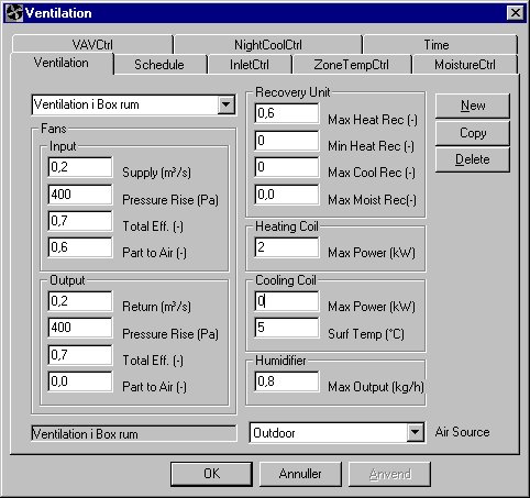
Ventilation system components
The system component dialog shows the components, which can be specified for the system. In this example data are specified for fans, recovery unit and a heating coil and furthermore a schedule for the system must be defined. Data for this example is inputted as indicated in the figure above.
Fans
Under the Fans group, the inlet and extract fans are defined by air-flow, pressure rise as well as total efficiency. Pressure rise and efficiency are used for calculation of the sum of the power requirement for the two fans according to the following formula:
\[ P = \frac{q_v \cdot \Delta p_t}{\eta_{\text{tot}}} \tag{1} \]
P is the power of the fan, W
qv is the air volume flow, m³/s
Δpt is the pressure rise over the fan, Pa
ηtot is the total efficiency for fan, motor and transmission.
The temperature efficiency for the recovery unit is entered as 0.6 in the Max Heat Rec field. The value 0 is entered in the remaining fields. A prerequisite for setting the Min heat rec. efficiency to 0 is that the system can be controlled so heat is not transferred from extract air to inlet air, when this is not needed (or wanted, e.g. during the summer). By "cooling recovery" (Max Cool Rec.) , the inlet air is cooled down, as it gives off heat to extract air (from the thermal zone). This function will normally only be relevant in buildings with mechanical cooling and presumes that the system can, in the event of a cooling requirement. When controlling the cooling recovery, the system checks that the extract air temperature is so much lower than the outdoor air that the desired heat transfer can take place.
The last parameter, Max Moist Rec. indicates whether moisture is transferred in the recovery unit, as is the case with regenerative recovery (e.g. rotating exchangers) as against recuperative recovery (e.g. coil exchangers).
Heating coil
The model for the heating coil is very simple, and is described by just one parameter, namely the maximum power output Max power, which can be given off to the air. Here the value 2 kW is entered.
Each of the components in a ventilation system are to be considered as components in a catalogue, so that each defined component can be used in several different systems.
Note that in a simple model with only one ventilation system, the automatically assigned component names can be used without any problem.
The last field on this tab, the Air Source indicates, from where the actual ventilation system gets its inlet air. The field is a selection menu showing all thermal and virtual zones as well as other ventilation systems of the model. The air can thus come from any of these sources and as a default it is assumed that the air comes from the virtual zone 'Outdoor', which is the case in this example.
Schedule and control for ventilation system
In the schedule it is possible to specify 5 different forms of control:
| Regulation type | Description |
|---|---|
| Inlet control (InletCtrl) | is a control, where the inlet temperature can be defined as a function of time and/or outdoor temperature. |
| Zone air control (ZoneTempCtrl) | where the inlet temperature is adapted (within chosen min. and max. values), in order to achieve the set-point of the room sensor. |
| Moisture control (MoistureCtrl) | which is primarily used in connection with dehumidification of the indoor air. The inlet air is dehumidified in the cooling coil, when the room's relative humidity exceeds the room hygrostat's set-point. This control can be combined with heating to a desired temperature set-point as well as humidification of the inlet air. |
| VAV control (VAVCtrl) | where the inlet air can be increased above the nominal as regards keeping the temperature (down) to a desired set-point. This control type is normally used when cooling is required. |
| Night cooling (NightCoolCtrl) | often combined with one of the others (different controls within different time definitions). With this control, the ventilation is started up (on/off) when the indoor temperature exceeds the set point to a certain degree (defined by the user). Though only in so far as the indoor temperature at the same time exceeds the outdoor temperature to a certain degree so that the indoor temperature will be reduced by means of night cooling. Via an entry in the control dialog it must be specified which components that are active during night cooling, so that, for example, it can be assumed that the cooling coil (the mechanical cooling system) is not in operation during night cooling. |
In principle, different forms of control can be used within the various time definitions, as a new control strategy is selected by first creating a new Schedule and then clicking Use this.
Data for control in the example
The control for the ventilation system is specified via the Schedule tab in the Ventilation component dialog. In any of the control strategy tabs it is possible to define a control strategy to apply to the ventilation system. In the actual example, the type "InletCtrl" is selected. This form of control is pure "steering", i.e. without any return message regarding conditions by the feeler to that which is being controlled, namely the ventilation components etc. in the system.
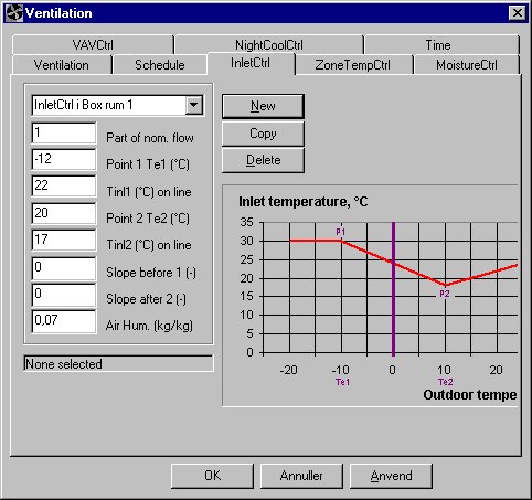
In the first field of the dialog Part of nom. flow it can be indicated that within the connected time definition, it can only operate with a certain share of the "nominal", which is defined under ventilator. This will, for example, be a simple way of defining the control for a system which runs with reduced air quantity at night-time. By means of the following 6 parameters in the dialog, the control curve for the inlet temperature is described.
In this case the inlet air temperature is controlled so that it is 22 °C when the outdoor temperature is -12 °C, dropping linearly with rising outdoor temperature to 17 °C at an outdoor temperature of 20 °C. When the outdoor temperature is below -12 °C or above 20 °C, the inlet temperature is constant, respectively 22 °C and 17 °C (slope of the line for the control curve outside these values is 0).
The last parameter in the dialog Air Hum. is only of significance for systems with a humidifier. As the field must not be empty, just any value for the absolute moisture content of the air is entered, e.g. 0.007 (kg water vapor / kg dry air).
The defined control form is selected by clicking the Apply button.
A description of the different control types is given in the section entitled Ventilation systems.
Save building model
All the data for the building have now been entered, and the model must therefore be saved. Before doing so, a control should be carried out to ensure that the model is complete by clicking the ModelList icon at the toolbar. If errors or deficiencies are found in the data, the program will give information about these, and otherwise all the data are (formally) in order. At the start of this example, the model's name was defined as "EX3" and the model must now be saved again under this name by clicking on the Save entry in the File-menu (shortcut: Ctrl+S).
Simulation
A simulation is now to be undertaken in order to compare the indoor climate and energy consumption for the new model (EX3) with that of the old model (EX2).
Selection of parameters in "hour-log"
By copying the model from EX2 over to EX3 (at the beginning of example 3) in addition to copying data for the current building model (the file EX3.DIS) also information (data) regarding hour-log, parameter lists etc. were copied into a new file named EKS3.G97.
As the simulation period is already defined from EX2, simulation can be started by clicking the Start-button at the Simulation tab of tsbi5. The simulation can be started by clicking the Start-button at the Simulation tab of tsbi5.
Results
The best overall view of the results of the calculations is normally obtained by analyzing the energy balance (HeatBalance) for the building or for the individual thermal zones.
Select "period" in the Time scale selection-menu (the first selection-menu counted from left), to obtain the heat balance for the whole simulation period, in this case the whole year. An energy balance will be shown, in which all contributions to the balance are indicated for the selected period. The statistics also show for how many hours of the year the operative temperature is below 20 °C and how many hours it exceeds 21, 24 respectively 26 °C (standard values for the temperature limits).
An overall view of the indoor temperature sequence can be obtained by selecting a "graphic" printout of the operative temperature OpTmp via the Tables tab.
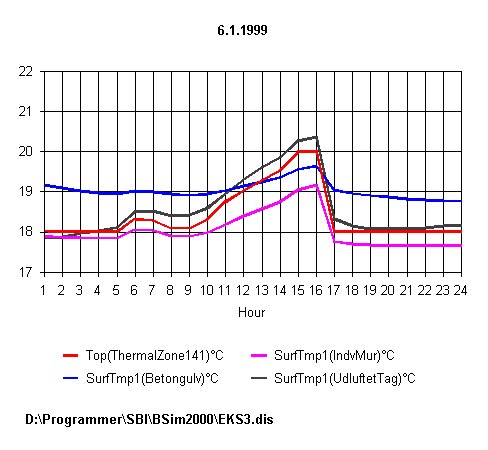
Analysis of the temperature variation over the whole day
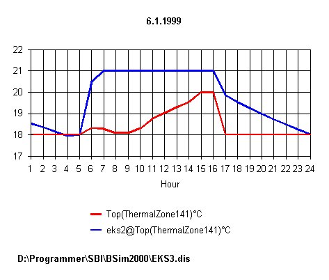
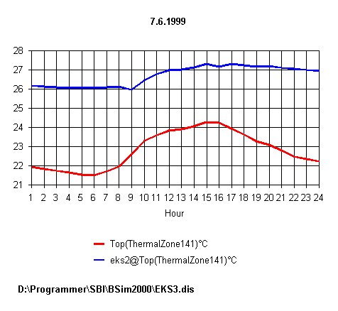
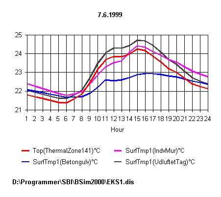
A closer analysis of the 24-hour temperature sequence is shown in the screen prints below for a day in week 1 and a day in week 23. Here, both the operative temperature and the surface temperatures of the internal walls, the ceiling and the floor are printed out.
Comparison of EX2 and EX3
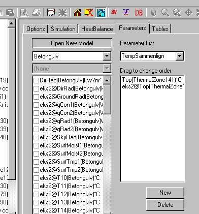
It is possible to create parameter lists with parameters from different models so that, for example, it is possible to compare alternative project solutions. In this case the thermal indoor climates in EX2 and EX3 are compared.
Clicking the New-button, at the Parameters tab creates a new parameter list. In this case, the name "Temp-compar" can be used for the list. By clicking in the groups (above the left window) a list of parameter groups is revealed as usual. From this the parameters from the actual model (EX3) can be selected. Here the group 'Indoor' is selected and the parameter operative temperature OpTmp selected.
A simple comparison is now desired of the sequence of the operative temperature in EX3 and EX2. In order to select the result parameters from EX2, click the Open New Model-button and a summary will appear of the models in the current path for which a result file (file type *.G97 ) is present. It is only possible to compare results from models located in the same path as the actual model.
By clicking on the model name "EX2" this model is selected, and parameters can be chosen here as normally. In the case shown, the OpTmp parameter from EX2 has been selected. A simple parameter list has thus been created from the two models, and both schedule and graphic printouts of the hourly values can be carried out as usual. The parameter names from the "strange" model are indicated in the parameter list with a preceding model name and a "@" in advance of the parameter name.
Printouts for a summer day and a winter day of the operative temperature and surface temperatures for the two examples. It can be seen that the program assigns each of the selected models a number, so that model EX3 corresponds to the parameter name and EX2 corresponds to ex2@ plus the parameter name.
The selected winter day is a day with high solar radiation and it can be seen that in EX3, the temperature exceeds the set point of 21 °C, because there is no shadow from neighboring buildings and the windows have no solar shading. For the selected summer day, the temperature in EX2 is 3 degrees higher than found in EX3, because solar shading, venting and ventilation have been defined in EX3.